Using Lidar point clouds for Orienteering base map generation

Added 31 May 2013: All the programs can be downloaded here!
Update 16 Aug 2013: Mindaugas Andrulis helped locate a bug where the scripts failed if the Easting values required 7 digits.

This article is based on my work with the base maps for JWOC 2015 in Rauland/Telemark Norway.

Laser scanning (Lidar) has caused a revolution in the quality of base material available for mapping, up to now however this has mostly been limited to defining a ground surface and then use it to generate contours with a fairly heavy amount of smoothing. I.e. here in Norway these contours, with 1 and 5 m intervals have been available to mappers as SOSI or Shape files.

The latest versions of OCAD have incorporated a LAS processing pipeline for Digital Elevation Model (DEM) and contour generation, initially this sw scaled very badly so that it was impossible to handle very large areas like I needed for the mountain areas in Rauland: I had to split my map into about 25-30 separate blocks, process them individually and then merge the results. This took a very long time (several weeks) and resulted in a base map with glitches in the contours along all the block boundaries. I spent some time in 2012 looking over the OCAD source code, suggesting ways to make it faster and/or scale better, and the latest updates to OCAD 11 has implemented one of those approaches so that it is now possible to import many sq kms of Lidar points.

In Sweden Jerker Boman wrote OL Laser a few years ago, this program is free and it allows better control of the contour generation process. It can also generate slope angle images and detect very steep areas as possible cliffs. Jerker implemented a batch processing pipeline for OL Laser so that it could be used for big jobs, but I had some stability problems and the boundary glitch problem remains.

Over in Finland Jarkko Ryyppö (of RouteGadget fame) made a big breakthrough with his "Map Machine" (Karttapullautin) which handles everything from the input Lidar data to a finished training map image which can be used as-is.

The solution I ended up with was to use the free LAStools programs developed by Martin Isenburg: Martin is the inventor of the LAZ format which can compress Lidar data by almost an order of magnitude, the reference implementation of the compression algorithm has been published as open source. LAZ is the format which is being used by most countries who have started to publish their Lidar databases, like Finland and the US.

Martin has written a set of extremely efficient utility programs (for Windows) that can be used freely by individuals and non-profit organizations to perform advanced Lidar processing on smaller data sets, I ended up using a few of his programs in a batch pipeline, with several helper programs written in perl that control the process and perform any extra processing. (I used the free Windows perl version from Activestate.com since it has very good library support.)

lidar-batch.bat

This batch file is started from the command line, from the directory where all the finished files should be generated, i.e. if all the LAZ files are located in the "base" subdirectory of the "norefjell" directory, the relevant command would be something like this:

c:\data\norefjell>lidar-batch base\*.laz

The result after a few minutes (depending upon project size) is a set of .dxf and .asc files ready for import into OCAD along with a set of Background Map images as detailed below.

Batch processing stages

Tiling the input data

lastile takes a set of las/laz files and splits them into individual tiles, each is sized 250x250 m, with a guard buffer of 35 m around all the sides, i.e. each tile will contain all the points from a 320x320 m square. The boundary area is very important since it allows all the subsequent operations to work independently while avoiding glitches or artifacts along the tile boundaries!

lastile -i %1 -tile_size 250 -buffer 35 -o tiles_raw\tile -olaz

Ground point determination

Here in Norway Lidar point clouds have already been classified as either Ground or Non-ground so I can use them as-is, otherwise LAStools has the lasground program which can do a pretty good job of figuring out what is ground and what isn't. (If your Lidar files haven't been ground classified you can use lidar-batch-ground.bat instead, this batch file adds an extra stage using lasground.exe to differentiate between ground and non-ground points.)

Lidar Vegetation Classification

The LAS standard has classifications for 4 different heights, i.e. Ground (2), Low Vegetation (3), Medium Vegetation (4) and High Vegetation (5), but with no fixed specification of which heights belong in each class, i.e. this is up to us as mappers to determine. For orienteering any points less than 30 cm above the ground will probably be noise in the form of low heather or tufts of grass, while any brush that is less than about chest height will impact runnability but not visibility so I chose to classify all points between 0.3 and 1.3 m as Low Vegetation.

Medium Vegetation is where the forest becomes dense, for both runability and visibility, so it determines where the map should have various levels of green, after some experimentation I ended up with the range 1.3 to 4.0 m for this class.

High Vegetation is everything above this, an area with only Ground and High Veg returns should normally be mapped as baseline white forest.

The LAStools program lasheight is used to perform this classification (I also drop any spurious points below -5 m and above +100 m):

lasheight -i tiles_raw\tile*.laz -drop_below -5 -drop_above 100 -classify_between 0.3 1.2 3 -classify_between 1.2 4 4 -classify_between 4 100 5 -odir tiles_classified -olaz -cores 4

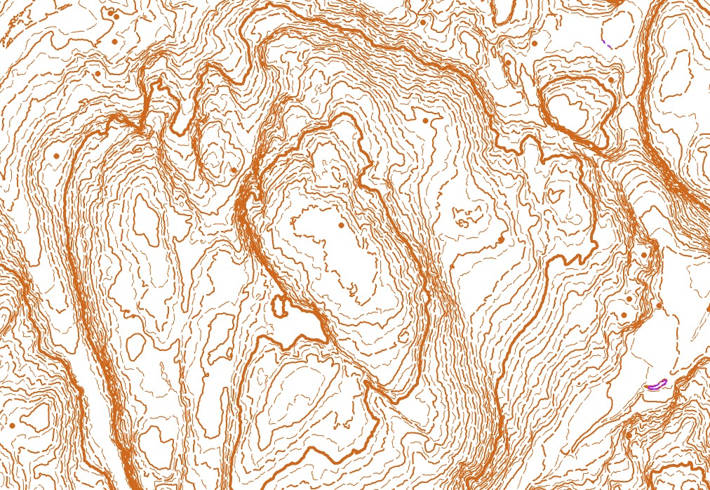
Contours, dot knolls and depressions

LAStools contains las2iso which can generate contour lines of several types and formats, I wrote a wrapper program in perl that calls las2iso to generate contours every 25 cm, which might seem excessive, but the idea is to first generate a very dense set of contour lines, then look for triple rings, i.e. contour loops that contain exactly two internal loops:

gen-dxf-iso-dep.pl -cores 4 -force tiles_classified\tile*.laz

contours, dot knolls and depressions

Such a triple ring can either indicate a low knoll (if the contours have increasing altitude) or a depression (if they drop down). I use the size of the outermost loop to determine if and how the knoll or depression should be mapped: A dot knoll has to be below a maximum size, otherwise it should be mapped with regular contours, while for a depression the size determines if it can be shown with a (negative) contour plus slope line(s) or as a point depression.

After this stage I remove all contours that should not end up on the final base map. By default I generate 4 classes of contours (25 m index, 5 m normal, 2.5 m form line and 1.25 m extra form line) since this makes it easy to hide/reveal one or more class. The number of contour classes and intervals between them can of course be configured, as long as they are all a multiple of the baseline 25 cm set.

Before I merge the individual tiles together I crop each set of contours so that only the central 250x250 m is left, then after merging I look for and splice together all contour segments that cross a tile boundary, i.e. making sure that each contour line will be a single OCAD object.

The result of this processing is a file named by the map project directory name with the suffix "_contours.dxf", i.e. "norefjell_contours.dxf" for the Norefjell project, along with a "norefjell_contours.crt" file which describes the mapping from DXF to OCAD object types.

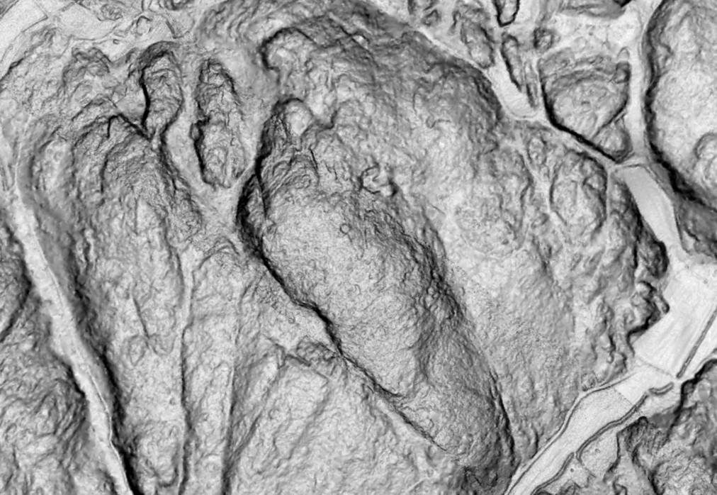
Digital Elevation Model and slope angles

las2dem is called from another perl program in order to generate tile-based DEM and slope files in .ASC format, merging the tile results into
a single elevation ASC file (which OCAD knows how to import) and a grey-scale slope file in GIF format (plus a GFW georeferencing "world file" so that the background image will end up in the correct spot).
slope angle image

gen-slope-asc.pl -cores 4 tiles_classified\tile*.laz The results are files named with "norefjell_elevation.asc" for the DEM data and "norefjell_slope.gif" for the slope angles.
The slope angle data is also used to generate a set of 4 black & white cliff images (cliff, cliff1, cliff2, cliff3):

If the vertical drop is steep enough it is shown as a black cliff, otherwise as white background:

cliff3 corresponds to 3+ m vertical drop over 1 m horizontal distance,
cliff2 is for 2-3 m drops and
cliff1 for 1-2 m,
while the "norefjell_cliff.gif" image is the sum of these three, i.e. any drop above 1 m.

Any of these images can be loaded as a transparent background map.

Vegetation classification for Orienteering

I use las2txt in pipeline modus in order to convert each compressed binary .laz tile into text format, then I accumulate the number of points from each of the four relevant classes (Ground/Low/Med/High Veg) that hit in each 2x2 m square. After trying many different classifiers I ended up with a model where I look for the 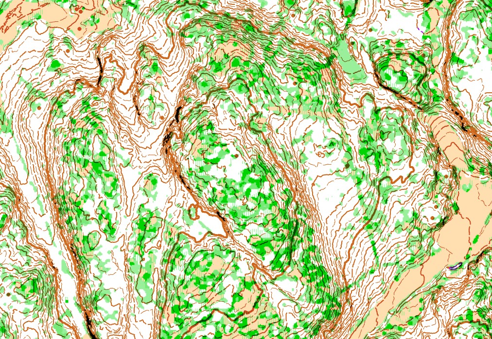vegetation and cliffs

relative distribution of points in each height group. In order to get significant results I needed to average the distribution over a circle centered on each square, the averaging is weighted so that the central points are more significant, dropping down to zero about 5 m away.

gen-laz-vegm.pl -cores 4 tiles_classified\tile*.laz

The results of this can be very noisy, changing classification for every 2x2 m block, so I have to filter them with a second low-frequency pass, this was based on an idea from Jarkko Ryyppö's mapping generator which also employs a two-stage process.

In my code I use a simple majority vote for a center-weighted area around each block: Whichever classification is most common wins.

The result is named "norefjell_vegetation.gif"

Vegetation classification feedback

Initially the various classes (white/yellow/stripe green/light/medium/dark green) is based on a set of trial-and-error tests I made, but after the first few surveying trips in the forest I found a general way to improve this:

I picked a number of locations in the forest that were typical for the various classifications, then put those benchmark spots into a specific file:

611548,6546040,G611626,6546550,Y611736,6546450,W611958,6546282,DG612116,6546686,WS ... "vegetasjon_facit.txt"

The codes stands for Green, Yellow, White, Dark Green and White with green Stripes. I can also use LG and YS for Light Green and Yellow with green Stripes.

If this file exists in the current directory the perl program will pick it up: On the first processing run the statistical distribution for each of the benchmark areas is calculated and the "vegetasjon_facit.txt" is updated, appending the percentage of each type of return (Ground/Low/Medium/High).

On subsequent runs these benchmark values are used, so that for each 2x2m spot in the terrain it will look for the benchmark spot which is most similar and use that classification. It is of course possible to iterate this process, so when you find one or more areas that are wrongly classified, they can be added to the benchmark file before restarting the gen-laz-vegm.pl program.

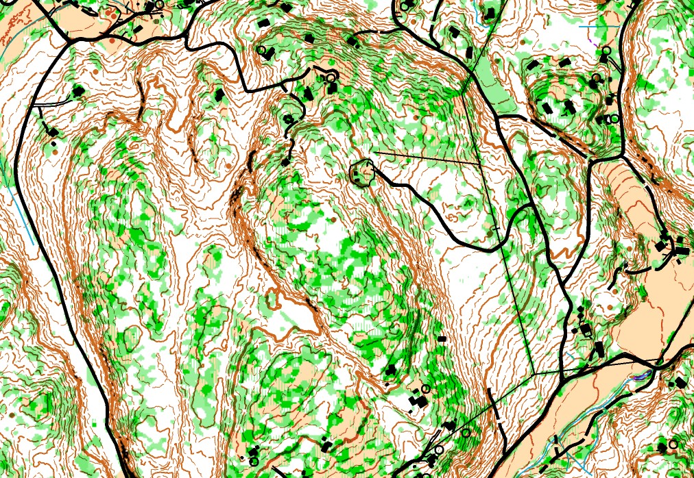
Adding public mapping data

Norwegian mapping data is stored in the SOSI format, this is a text-based format which (as far as I know) is used only in Norway. It is however very self-descriptive, with all coordinates stored in UTM with cm resolution, so it was fairly easy to write a sosi2dxf.pl program which converts most object types to the corresponding OCAD objects.

I received a lot of help from Gian-Reto Schaad (from OCAD AG) here, coming up with several improvements to the DXF import process so that I can get elevation data for any line or point object (like contour lines and dot knolls) as well making it possible to import area objects which contains holes, i.e. a lake with one or more islands.

Adding this results in vector data for roads, buildings, some area use boundaries, power lines, rivers and creeks as well as some paths. At this point the base map is ready for field surveying:

finished base map

All the programs I have developed and listed here are hereby released for free use/modification by anyone interested in orienteering mapping. I would appreciate getting an email with a copy of any map generated this way!

Oslo, May 30 2013
Terje Mathisen
terje.mathisen(at)tmsw.no

PS. All the map samples shown are from a separate project, mapping the Hvaler archipelago in the Oslo fjord. See Asmaløy and Hvaler for the work in progress.